Multiple Linear Regression from Scratch


The code for this project is available on my GitHub.
Logistics
This is my first “from scratch” machine learning project, so there are a few logistical things I had to resolve:
- Should I use Jupyter Notebook or Visual Studio Code?
- Both! It looks like Jupyter Notebook is great for visualizations, but I like VS Code’s extensions. I’ll edit my notebooks in VSC.
- Why do so many people write linear regression as a class instead of a bunch of functions?
- Reusability, namespaces, and inheritance. Instance variables, too, but that doesn’t seem to matter too much for linear regression.
- This Reddit post expands on the benefits of classes.
- Reusability, namespaces, and inheritance. Instance variables, too, but that doesn’t seem to matter too much for linear regression.
- I don’t know how to create a class in Python. What do I do?
- The official documentation actually does a pretty good job of explaining classes.
- Where do I get my training data set?
- There’s the famous Boston Housing Dataset, but I opted for the “House Prices - Advanced Regression Techniques” dataset from Kaggle. I still need some guidance on implementing this from scratch, so I’m roughly following Venelin Valkov’s Medium post when I get stuck. He uses the Kaggle dataset, so I will, too.
- Why not make your own data set?
- I think real-world data is more meaningful. I understand learning to synthesize data is very important, especially in CV, but I’m not advanced enough for that—yet.
- How do I validate my model?
- I’m going to use PyTorch! Might as well learn one of the most popular ML libraries along the way.
Visualizing the Dataset
First, let’s import some libraries:
import numpy as np
import matplotlib.pyplot as plt
import pandas as pd
import seaborn as sns
We want to have an idea of what the dataset is like. I’m covering the very basics of this since it’s not the main goal of this program (coding linear regression).
We can import the dataset (above) and look at the first three rows of data:
df_train = pd.read_csv('./house-prices-advanced-regression-techniques/train.csv')
df_train.head(3)

Note that we’ll have to use feature scaling because our feature values are pretty different. LotFrontage and LotArea are already off by magnitudes of 100. Even if they weren't, we'd still normalize because it’s good practice.
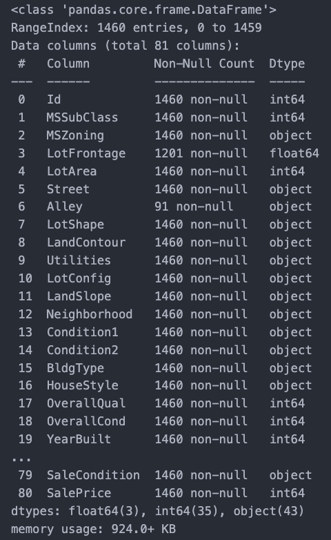
This doesn’t tell us too much about the data types we have, though. Another way we can look is with the .info() method.
df_train.info()
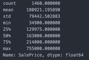
Since I’m just trying to get a basic understanding of linear regression, I won’t be using all 80 features. Let’s take a closer look at what we’re trying to predict: SalePrice.
df_train['SalePrice'].describe()
And a plot helps.
plt.figure(figsize=(15,6))
sns.histplot(df_train['SalePrice'], color='b', bins=100)
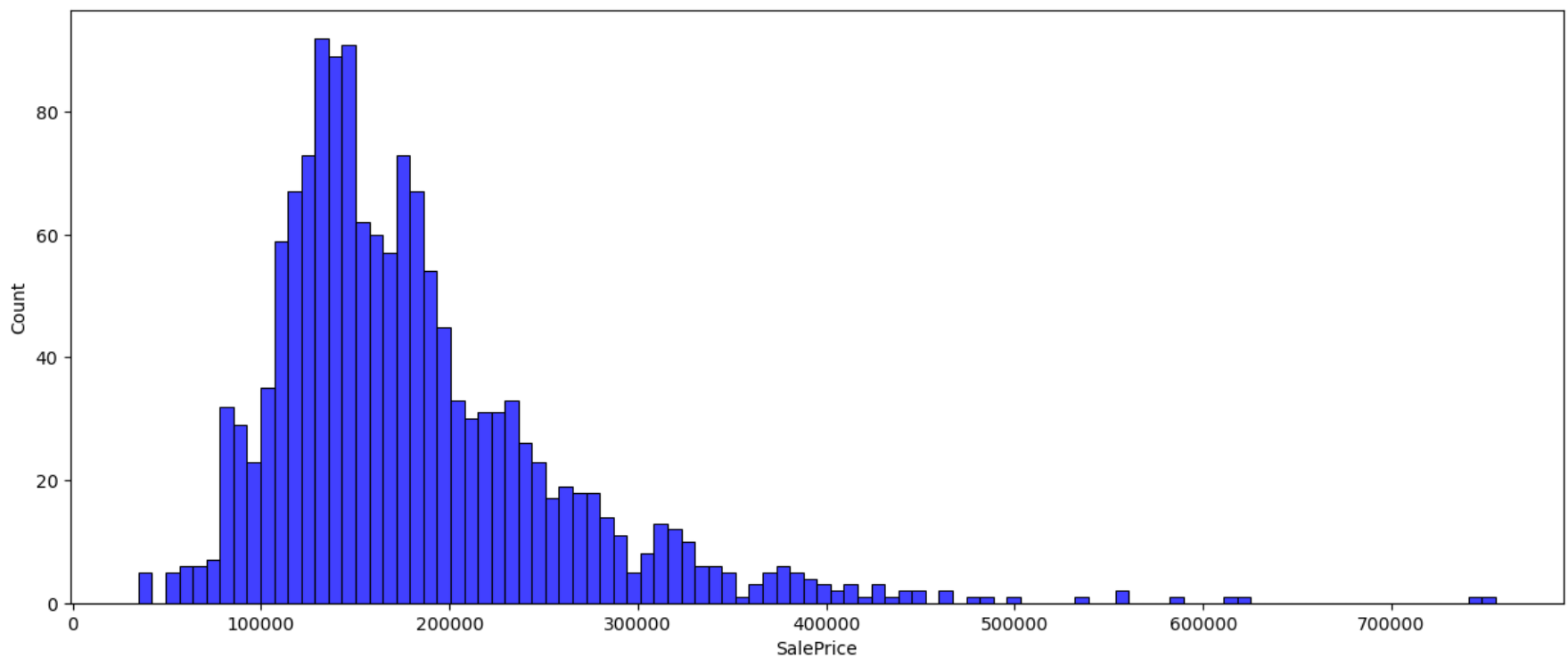
So, we can probably expect most of our predicted housing prices to be in the range of 100k to 300k.
Feature Scaling
We’ll scale our features using mean normalization:
\[x’ = \frac{x - \mu}{\max(x) - \min(x)}.\]
def mean_normalization(arr):
    normalized_arr = (arr - np.mean(arr)) / np.ptp(arr)
    return normalized_arr

def mean_normalization_y(arr):
    max_y = np.max(arr)
    min_y = np.min(arr)
    avg = np.mean(arr)

    normalized_arr = (arr - avg) / (max_y - min_y)
    return normalized_arr, max_y, min_y, avg
I’m creating a separate normalization function for our label y because we’ll need to store the max, min, and mean to convert from normalized values to actual prices.
Then, we normalize whatever features we want to use. I chose FullBath, LotArea, and YearBuilt randomly. There are better ways to choose features, but again, I’m just trying to implement linear regression. Make sure you normalize SalePrice, too.
You should have something like this:
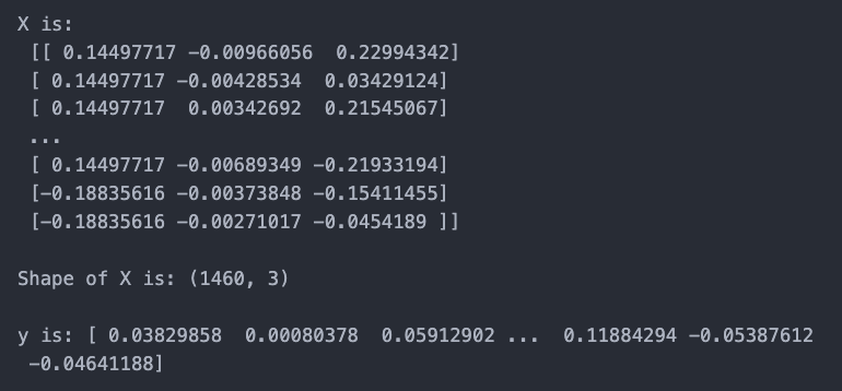
X is an m by n matrix, where m is the number of training examples and n is the number of features. y is an n by 1 vector.
Implementing Multiple Linear Regression
class LinearRegression:
    def __init__(self):
        self.weights = None
        self.bias = None

    def gradient_descent(self, X, y, epochs, learning_rate=0.01):
        m, n = X.shape
        self.weights = np.zeros(n)
        self.bias = 0.0

        epochCosts = []

        for i in range(epochs):
            # Find predicted values
            f_wb = np.matmul(X, self.weights) + self.bias

            # Calculate cost
            err = f_wb - y
            cost = np.sum(err**2) / (2 * m)
            epochCosts.append(cost)
            if i % 50 == 0:
                print(f'The cost at epoch {i} is: {cost}')

            dJ_dw = np.matmul(X.T, err) / m
            dJ_db = np.sum(err) / m

            self.weights -= learning_rate * dJ_dw
            self.bias -= learning_rate * dJ_db

        return self.weights, self.bias, epochCosts # return weights, bias, costs for graphing

    def predict(self, X):
        return np.matmul(X, self.weights) + self.bias
For each training example, our model multiplies a weight parameter with its corresponding feature value for that training example. Then, we add a bias. This is very similar to the classic $y = mx + b$ formula.
$$f_{\vec{w}, b} (\vec{x}) = \vec{w} \cdot \vec{x} + b$$
The output of our model is the estimated price (except it's normalized, so it won't actually be the price).
At first, this model will be very inaccurate. It doesn't know what our parameters $w$ and $b$ should be. So, we use gradient descent to find the correct values.
We calculate how "off" our model is by using the Mean Squared Error (MSE) cost function $$J(\vec{w},b) = \frac{1}{2m} \sum_{i=1}^m (f_{\vec{w}, b}(\vec{x}) - \vec{y})^2,$$ where $\vec{y}$ is the correct values for our training examples. Note that the cost function is the sum of the errors for all $m$ training examples.
Then, we'll do gradient descent:
$$\vec{w} = \vec{w} - \alpha \frac{\partial J}{\partial \vec{w}}$$
$$\vec{b} = \vec{b} - \alpha \frac{\partial J}{\partial \vec{b}},$$
where our partial derivatives are given by
$$\frac{\partial J}{\partial \vec{w}} = \frac{1}{m} \sum_{i=1}^m (f_{\vec{w}, b}(\vec{x}) - \vec{y}) \vec{x}$$
$$\frac{\partial J}{\partial \vec{b}} = \frac{1}{m} \sum_{i=1}^m (f_{\vec{w}, b}(\vec{x}) - \vec{y}).$$
We'll perform gradient descent on all $m$ training examples for a number of times defined by epochs in the code above.
One thing to note: When computing dJ_dw, we have to take the transpose of X when we perform a matrix multiplication with that and err because err has dimensions m by 1.
Our predict() function just returns $f_{\vec{w}, b}(\vec{x})$ since this tells us the normalized price for the input matrix X.
If we run this model on the matrix X from above and graph our cost, we get this cost function:
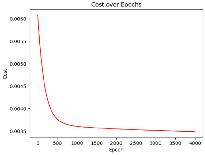
Looks good! Our cost always decreases.
Predicting Housing Prices
We’ll use our model to predict housing prices of the test dataset. Unfortunately, I don’t have access to the correct labels. That’s okay! We’ll compare our model to PyTorch’s linear regression model. Hopefully we’re not completely off.
Using the process shown above, we’ll create the matrix X_test with all of our testing data, isolating only the features we chose for our model.
Then, we run our prediction:
predictions = model.predict(X_test)
# Convert predictions to dollar values
predictions = predictions * (max_y - min_y) + avg
print(predictions)

Looks reasonable. At least from the values we can see, the prices of these houses are within the expected range of 100k-300k.
Testing the Model Against PyTorch
(This section was heavily influenced by Patrick Loeber’s Linear Regression video on YouTube.)
Let’s import the necessary dependencies:
import torch
import torch.nn as nn
Then, we’ll build our model:
X_torch = torch.from_numpy(X).float()
y_torch = torch.from_numpy(y.reshape(-1,1)).float()

input_size = X.shape[1] # Number of features
output_size = 1 # One value, the price of the house

model = nn.Linear(input_size, output_size)

criterion = nn.MSELoss() # Defines the loss function
optimizer = torch.optim.Adam(model.parameters(), lr=0.05)

# Training
epochs = 4000
for epoch in range(epochs):
    y_hat = model(X_torch)
    loss = criterion(y_hat, y_torch)

    loss.backward() # Backprop

    optimizer.step() # Updates weights
    optimizer.zero_grad()

    if epoch % 50 == 0:
        print(f'The cost at epoch {epoch} is: {loss.item():.4f}')
PyTorch uses PyTorch Tensors, so we have to convert our training data from a NumPy array to a tensor. Then, we specify our input_size and output_size because PyTorch needs those arguments to create our model.
We’ll define the loss function as the MSE function like we did above. We’ll also define our optimizer as the Adam optimizer. We didn’t do this in our model because it’s harder to implement. The basic idea of the Adam optimizer is as follows:
With our model, we had a constant learning rate $\alpha$. With the Adam optimizer, the learning rate changes based on how big of a step gradient descent needs to take. This makes gradient descent work faster than our model that uses a constant learning rate. (We define the lr=0.05 as our initial learning rate. The model needs to start somewhere. This is similar to how our regression model defines our initial weights and bias as 0.)
Then, we train the PyTorch model. This model uses back propagation to calculate partial derivatives, whereas we brute force it using forward propagation. In practice, back prop is much better.
After we update our weights, note that we have to call optimizer.zero_grad() so our gradients for the next epoch start out as 0 (which the model will then calculate the correct gradient for that epoch and update the weights with optimizer.step()).
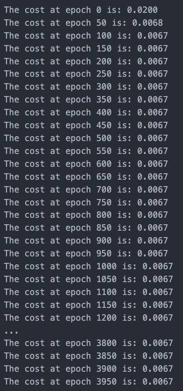
The cost function converged in 100 epochs, compared to our model’s need for about 1000 epochs for convergence!
We predict housing prices on our dataset using the PyTorch model as we did above. Then, let's graph our predictions on the testing dataset:
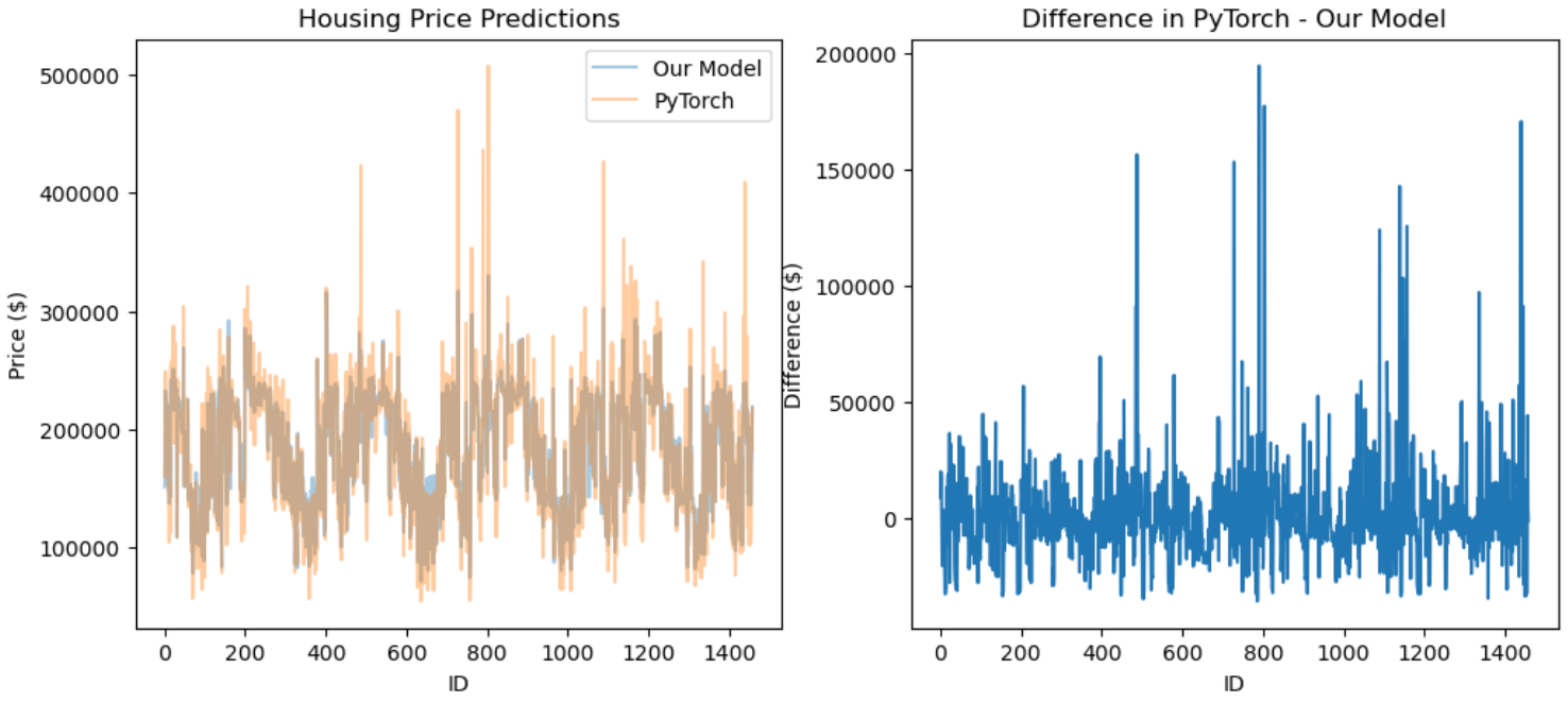
It looks like our model captured the general trends that PyTorch did, but there were still some pretty big differences. That’s okay for now! General trends are enough to show that our model works correctly.
Like this tutorial? Subscribe to my weekly computer vision newsletter for more!
No spam, no sharing to third party. Only you and me.
Member discussion